Missing values can cause bias. So most books introduce imputation methods like mean substitution or LOCF(Last Observation Carried Forward). But in this post, I will explain why people say unconditional mean substitution is bad with a simple example.
Mechanisms of Missingness
Little and Rubin(2002) categorized missingness into three categories.
- MCAR(Missing Compmletely At Random)
- MAR(Missing At Random)
- NMAR(Not Missing At Random)
In simple terms, MCAR is missing unconditionally random, MAR is missing conditionally random. And NMAR is neither of the both.
Here is a (unrealistic, but) simple example model.
\[\textrm{Weight} = 0.48 \times \textrm{Height} + e\]
I will cover only the missing weight values in this post. Assume that we can somehow find out what the real value is even if it is missing.
If missingness of weight is not related to other variables including itself, it is called MCAR. It is like missingness is totally determined by flipping coins.
If missingness of weight is conditional on height(and other variables in the model) but independent of the weight value, it is called MAR. Overall distribution of weight can be different dependent on missingness, but given the information of height(and other variables in the model), it is identical. Missing is independent of weight, given the height(and other variables in the model). Given the height (and other variables in the model), missing occurs independent of the height. So we can say missingness is determined by flipping coins conditional on the value of the height(and other variables in the model).
If we digest the above using some of the basic probability rules, we get to the conclusion below.
Missing value distribution is not different from observed value distribution, given the value of other variables in the model.
The following might be true.
\[p(y|y_{\textrm{missing}}) \neq p(y|y_{\textrm{observed}})\]
But the following holds true.
\[p(y|y_{\textrm{missing}}, x_1, x_2, \cdots, x_p) = p(y|y_{\textrm{observed}}, x_1, x_2, \cdots, x_p)\]
It is like flipping coin again. But it could be a different coin for different value of explanatory variables.
If it is neither MCAR nor MAR, it is called NMAR. For example, if the missingness of weight is dependent on weight itself, it is NMAR.
For predictive models, it is sufficient of check if missingness is random conditional on other observed variables. But for causal model, we should consider if there is unobserved variables that might cause or be related to missingness. For now, I will consider only predictive models.1
- [AD] Book for R power users : Data Analysis with R: Data Preprocessing and Visualization
Why not just use complete data?
The main problem is the bias introduced by missing data. As the number of missing increases, the bias could be huge. Another problem is decreasing sample size. Smaller sample size means less power.
How was missing data handled, traditionally?
- Listwise Deletion : Use only complete data
- Pairwise Deletion : Use all data available for each analysis
- Unconditional mean substitution
- Regression Imputation(Conditional mean substitution)
- Stochastic Regression Imputation
- Hot-Deck Imputation
- Last Observation Carried Forward
Listwise Deletion means using only complete data. Ignore any data with at least one missing.
Pairwise Deletion means using all available data for each estimates. Let’s say we need to compute covariance matrix of variables \(X_1\) , \(X_2\) , and \(Y\) . We need to compute covariance of each pairs. We can use data missing in \(Y\) for computing covariance of \(X_1\) and \(X_2\) . This method can cause the problem of non-positive definite covariance matrix estimate.
Unconditional mean substitution imputes missing with the variable mean.
Regression Imputation utilizes regression analysis and impute missing with regression mean.
Stochastic Regression Imputation also uses regression analysis. It imputes missing with additional stochastic error term.
Hot-Deck Imputation imputes missing with values from other complete data. Wikipedia describes it as below.
A once-common method of imputation was hot-deck imputation where a missing value was imputed from a randomly selected similar record. The term “hot deck” dates back to the storage of data on punched cards, and indicates that the information donors come from the same dataset as the recipients.
Statisticians at the Census Bureau originally developed the hot-deck to deal with missing data in public-use data sets, and the procedure has a long history in survey applications (Scheuren, 2005; Enders, 2010).
Last Observation Carried Forward imputes missing with last observed value for the same group in the logitudinal data.
Which one of those missing data analysis above is unbiased depends on the whether missing is MCAR, MAR, or NMAR and what one is estimating using the analysis. For instance, for estimating a regression parameters \(b_1\) of \(y=b_0 + b_1 x_1\), listwise deletion is fairly appropriate for MCAR or MAR data, unless we care much about losing power. But estimating the mean \(y\) averaging only observed \(y\) could be seriously biased for MAR data if we use listwise deletion.
Deletion or imputation methods above result in complete data and we can use complete data analysis method. That’s why we prefer imputation or deletion more than other special methods developed for dealing with missing data.
Estimating mean \(y\) : MAR & listwise deletion
If \(y\) is missing complete random, estimating \(y\) using only observed data is okay because \(p(y|y_\textrm{missing}) = p(y|y_\textrm{observed})\) .
Estimating mean \(y\) : MAR & mean substitution
If \(y\) is missing conditionally random, using only observed data could be problematic because \(p(y|y_\textrm{missing}) \neq p(y|y_\textrm{observed})\) . Let’s say \(p(\textrm{missing}) \sim \textrm{height}\) . The probability of missing on weight increases as the height increases. In that case, the probability of missing weight is increased as the weight increases. So just using the complete data means deleting higher weight values and introducing a bias on estimating the mean weight.2
Estimating mean \(y\) : MAR & mean substitution
So we would better be using regression mean(estimated weight mean given the height). Using the conditional mean for missing data might lead to too small variance estimate but it is not biased.
- [AD] Book for R power users : Data Analysis with R: Data Preprocessing and Visualization
Simulation
Data
library(dplyr)
library(tidyr)
library(ggplot2)

# sample size 100
n <- 100
# height mean 170, std 15
h <- rnorm(100, 170, 15)
# true relation : weight =  0.48 * height
# given height, weight distribution N(0,7^2)
w <- 0.48 * h  + rnorm(n, 0, 7)

# weight population mean
w_pop <- 170*0.48 # 81.6
h_pop <- 170
# missing is dependent on height
w_missing <- runif(n, 0, 1) < (h-min(h))/(max(h)-min(h))

dat = data.frame(h=h,
                 w=ifelse(w_missing, NA, w),
                 w_complete = w,
                 w_missing = w_missing)

#dat %>% gather()
ggplot(dat, aes(x=h, y=w_complete, col=factor(w_missing))) +
  geom_point() +
  scale_color_manual(values=c('black', 'grey'))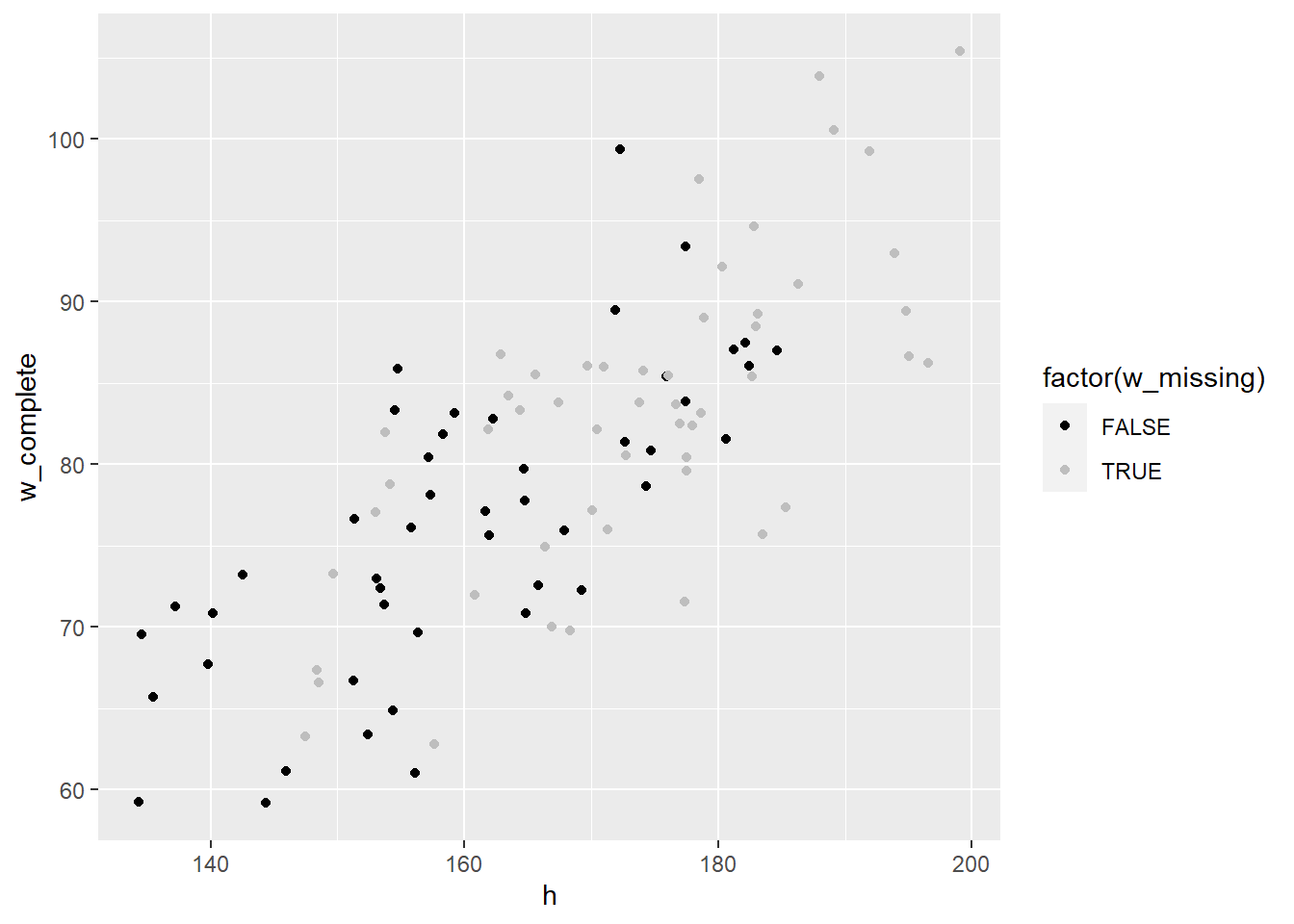
Listwise deletion
Estimated weight mean from using complete data seems biased.
## average weight?
mean(dat$w_complete)
## [1] 79.86512wmean_est = mean(dat$w, na.rm = TRUE)
wmean_est## [1] 76.49322t.test(dat$w)##
## One Sample t-test
##
## data: dat$w
## t = 58.46, df = 47, p-value < 2.2e-16
## alternative hypothesis: true mean is not equal to 0
## 95 percent confidence interval:
## 73.86092 79.12552
## sample estimates:
## mean of x
## 76.49322Mean substitution
Simple but bad alternative in terms of bias for MAR data is mean susbstitution.
w_mean <- mean(dat$w, na.rm=TRUE)
dat$w_imputed <- ifelse(dat$w_missing, w_mean, w)

wmean_est = mean(dat$w_imputed)
wmean_est
## [1] 76.49322res <- t.test(dat$w_imputed)
res##
## One Sample t-test
##
## data: dat$w_imputed
## t = 122.46, df = 99, p-value < 2.2e-16
## alternative hypothesis: true mean is not equal to 0
## 95 percent confidence interval:
## 75.25384 77.73260
## sample estimates:
## mean of x
## 76.49322The population weight mean is 81.6 but the estimated mean is 76.49. The confidence inteval is 75.25-77.73.
Regression imputation
We can use regression model to imput the missing values.
mod <- lm(w ~ h)
w_hat <- predict(mod, dat)
#w_hat <- coef(mod) %*% rbind(1,dat$h)
dat$w_imputed <- ifelse(dat$w_missing, w_hat, w)

wmean_est = mean(dat$w_imputed)
wmean_est
## [1] 79.89369res <- t.test(dat$w_imputed)
res##
## One Sample t-test
##
## data: dat$w_imputed
## t = 94.065, df = 99, p-value < 2.2e-16
## alternative hypothesis: true mean is not equal to 0
## 95 percent confidence interval:
## 78.20839 81.57898
## sample estimates:
## mean of x
## 79.89369Estimated weight value is 79.89, 95%-confidence interval is 78.21-81.58. Compare this with estimated weight mean from listwise-deletion.
mean(dat$w_complete)## [1] 79.86512t.test(dat$w_complete)##
## One Sample t-test
##
## data: dat$w_complete
## t = 81.261, df = 99, p-value < 2.2e-16
## alternative hypothesis: true mean is not equal to 0
## 95 percent confidence interval:
## 77.91499 81.81525
## sample estimates:
## mean of x
## 79.86512Here are some explanatory posts and a paper that show how the causal model can be beneficial to understanding missing mechanisms: Musings on missing data, Using causal graphs to understand missingness and how to deal with it, Graphical Models for Inference with Missing Data↩︎
In fact, simulation studies suggest that mean imputation is possibly the worst missing data handling method available(Enders, 2010).↩︎